Drawing scatterplots

The incenp.plotting.scatterplot module provides a scatterplot function to facilitate the creation of scatter plots.

Note that what I call a ”scatter plot” here may not be the most common acceptation of the term. I do not mean the 2-dimensional plotting of two variables (one on the x-axis, the other on the y-axis). Rather, I mean the plotting of a single variable on the y-axis, akin to a bar chart, but with all data points depicted as scattered dots.

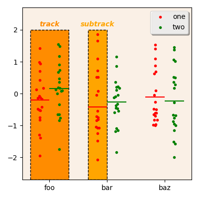
A sample scatter plot.

The figure above is a sample “scatter plot”. The orange boxes are not part of the plot, but have been added to illustrate what are tracks and subtracks in the context of the incenp.plotting.scatterplot module.

Sample data

The module is intended to work with indexed DataFrame objects (including multi-indexed DataFrame). Let’s create such an object, which we will use throughout this page:

index = pd.MultiIndex.from_arrays([
        ['foo'] * 40 + ['bar'] * 40 + ['baz'] * 40 + ['qux'] * 40,
        ['one', 'two'] * 80
    ],
    names=['first', 'second']
    )
df = pd.DataFrame(np.random.randn(160,4), index = index,
    columns=['A', 'B', 'C', 'D'])

This creates a DataFrame with 4 columns (A to D) and 160 rows, indexed in two levels (level first, with 4 distinct values foo, bar, baz, and qux; and level second, with 2 distinct values one and two).

Quick start

As an initial example, here is the call to scatterplot to draw the graph above (ax is supposed to be a matplotlib.axes.Axes object):

scatterplot(ax, df, columns='A',
            tracks=['foo', 'bar', 'baz'], trackname='first',
            subtracks=['one', 'two'], subtrackname='second')
ax.legend(['one', 'two'])

The columns parameter indicates that the values to be plotted comes from the column named A.

The tracks parameter gives the index values used to distribute the values of column A into three different tracks (one track for rows with index value foo, one track for rows with index value bar, and so on); the associated trackname parameter indicates which index level to use to lookup the values specified in the previous parameter, if df is a multi-indexed DataFrame.

The subtracks and subtrackname parameters are similar to the tracks and trackname parameter above, but for subtracks instead of tracks. Here, they are used to say that values from rows with index value one are to be plotted on one subtrack, while values from rows with index value two are to be plotted on another subtrack.

Playing with tracks, subtracks, columns

The following code will plot the same values as above, but will invert the tracks and the subtracks: the second-level index (second) will be used to distribute values along tracks while the first-level index (first) will be used to distribute values along subtracks:

scatterplot(ax, df, columns='A',
            tracks=['one', 'two'], trackname='second',
            subtracks=['foo', 'bar', 'baz'], subtrackname='first')
ax.legend(['foo', 'bar', 'baz'])

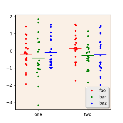
A scatterplot with inverted tracks and subtracks.

Values from several columns in the source DataFrame can be plotted at once, by giving a list of column names (instead of a single name) to the columns parameter. By default, values from each column are plotted in a different track. In the following examples, values from the columns A, B, and C are plotted; the first-level index is used to distribute values along three different subtracks; the second-level index is used to filter the DataFrame prior to plotting so that only rows with the index value one are plotted.

scatterplot(ax, df.xs('one', level='second'),
            columns=['A', 'B', 'C'],
            subtracks=['foo', 'baz', 'qux'], subtrackname='first')
 ax.legend(['foo', 'baz', 'qux'])

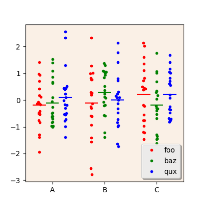
A scatterplot with values from several columns of the source DataFrame.

To plot values from several columns as different subtracks rather than different tracks, use the subtrackcolumns parameter as in the example below. The tracks and trackname parameters may then be used to define what goes into the tracks.

scatterplot(ax, df.xs('one', level='second'),
            columns=['A', 'B', 'C'], subtrackcolumns=True,
            tracks=['foo', 'baz', 'qux'], trackname='first')
ax.legend(['A', 'B', 'C'])

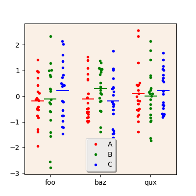
A scatterplot with values from several columns of the source DataFrame, plotted as separate subtracks.

Miscellaneous features

When plotting two subtracks, the testfunc parameter may be used to have the scatterplot function draws the result of a statistical test comparing the values from each subtrack in each track.

The value of the testfunc parameter should be a function accepting two DataSeries and returning a P-value, such as a the following wrapper around Scipy’s mannwhitneyu function:

from scipy.stats import mannwhitneyu

def do_mannwhitney(a, b):
    result = mannwhitneyu(a, b)
    return result.pvalue

Below is an example of using such a wrapper, with the resulting plot:

scatterplot(ax, df, columns='B',
            tracks=['foo', 'baz', 'qux'], trackname='first',
            subtracks=['one', 'two'], subtrackname='second',
            testfunc=do_mannwhitney,
            colors='cm')
ax.legend(['one', 'two'])

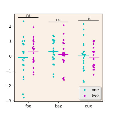
A scatterplot with results of statistical tests between subtracks.

The example above also shows the colors parameter, used to change the colors for the different subtracks. It can either be a string containing one-letter color codes, or a list of Matplotlib colors. The string or the list must be at least as long as the number of subtracks to plot.